NotesFrom a Small Universe
Ideas on space, time and causality.
Quantum Mechanics and Causality
This chapter is dedicated to quantum mechanics. Loosely speaking, quantum mechanics are the rules that govern how tiny objects such as atoms and subatomic particles behave. A lot of the results of quantum theory seem entirely counterintuitive, maybe even unphysical, when first encountered. But these results have been borne out by many, many experiments over the last century. We find here an example of our intuition failing us when we try to apply it to scales far smaller than those we deal with in our everyday lives. But of course it is these tiny atoms that make up the objects we deal with every day, and the counterintuitive results of quantum mechanics must apply at these scales as well. What this shows us is that some of the notions we draw from our intuitions about the nature of the universe are actually incorrect.
What is Temperature?
In order to understand the following sections we need to discuss what temperature is on a microscopic level. As you are probably aware, all objects are made up of microscopic atoms. Although an object may seem to be perfectly still the atoms within it are constantly moving. In a gas the atoms are free to move more or less wherever they please and swirl around like a swarm of insects. In a solid object the atoms are more constricted in their movements due to the chemical bonds between them that hold them in a more rigid structure. However, even in a solid, atoms still possess some movement, they are able to vibrate about their spot or ‘oscillate’.
The temperature of an object is a measure of the average speed at which the atoms in that object are moving. The faster the average speed, the higher the temperature. When an object is heated, that heat is giving energy to the object which will give the atoms more kinetic energy- the atoms move faster. If a hot object is placed against a cold object then where the two objects meet the atoms are able to collide. These collisions transfer energy from the faster moving atoms in the hot object to the slower moving atoms in the cold object and the temperature of the two objects will converge on a common value.
Blackbody radiation and Planck’s interpretation
Have you ever wondered why an object glows red hot or even white hot? All objects emit radiation right across the electromagnetic spectrum (see Fig in Relativity I), but how much is radiated at what wave lengths is governed by the temperature of the object. For example at human body temperature an object will emit mostly infrared radiation, a fact which makes people appear very bright in an infrared camera. In order to emit an appreciable amount of radiation as visible light the object’s temperature needs to be very much higher than human body temperature- a stove top needs to reach a few hundred degrees before it glows red and a filament light bulb needs to be at a temperature of a couple of thousand degrees in order to glow as it does.
The amount of thermal radiation an object gives off is called a blackbody spectrum, it looks a bit like a skewed bell curve across the electromagnetic spectrum with the exact shape determined by the object’s temperature. The name ‘blackbody’ is slightly confusingly since we tend to associate it with objects that are visibly glowing, it comes from the idea that a black object absorbs all the radiation that falls upon it before re emiting it. But why do objects give off radiation? And how is it dictated by their temperature? In the late 1800’s the subject was a hot topic in theoretical physics [1] and this work culminated around 1901 with the work of Max Planck. Planck had been seeking a theoretical description of how a blackbody spectrum arises, in other words why a human body emits mostly in the infrared but the hotter filament light bulb emits brightly in the visible spectrum. Planck drew his inspiration [2]. from the results of experiments carried out by Heinrich Hertz. Central to Hertz’s experiments was an invention of his called the Hertz oscillator, where a voltage was applied to a circuit with a very small gap. A spark would leap across the gap and generate an electromagnetic wave [A].
Crucially, Planck realised that Hertz had found a mathematical description for an object that emitted electromagnetic waves and that they could also, in principle, work the other way and absorb electromagnetic waves. Planck then looked at what would happen if you considered an object as being made up of a large number of these oscillators. These oscillators were later understood to be the electrons in atoms although atomic theory was not well accepted at the time least of all by Planck. All the same, we’ll use the modern language for our description. If an object was made up of atoms that acted like these oscillators then they could all interact with one another. That is to say the atoms could all absorb radiation put out from the others and then re emit it. How much absorption and emission went on would depend on the energy available, i.e. the temperature of the object. Could this give a sensible description of the real world where human bodies emitted in the infrared and hotter objects emitted in the visible light?
Planck found that the only way he could get his calculations to yield the correct amounts of radiation, as measured experimentally, was to restrict the frequencies at which the atoms could vibrate to certain, distinct values. To make up some numbers for an example, the atom might be able to vibrate at 100 times per second or 102 times per second but not 101 times per second or anywhere else in between.
When a given atom emitted radiation it lost energy and so it vibrated slower and conversely if an atom absorbed radiation it gained energy and vibrated faster. Because the atoms could only vibrate at particular values they could only ever emit or absorb radiation of particular corresponding values. An atom could emit radiation that dropped it from vibrating 102 times per second to 100 times per second but it could not emit radiation that dropped it to vibrating 101 times per second. Assuming then that it was vibrating atoms that produce radiation in the first place, this implied that radiation could only exist with certain, well defined energies. At the time Planck did not lay too much importance on this restriction, he considered it little more than a mathematical trick to make the theory work with little attachment to physical reality, assuming that a more satisfactory explanation would develop with time. Actually, this restriction was the genesis of quantum mechanics and would profoundly alter the way physics was done.
Einstein was intrigued by this idea that light from a system could only taken on certain frequencies (102 times per second say). It occurred to him that the most natural way to picture Planck’s system was if light was being emitted in little packets every time an atom changed the frequency of its vibration. If you considered a radiation field (a room filled with light, for example) to be made up of these packets then in many ways it was analogous to a gas made up of many individual particles. For example, if you took a small volume of air you could statistically guess how many particles you would count based on the temperature. Similarly, if you took a small volume of a radiation field you could statistically guess how many packets of radiation you would count based on the energy of the field. [B]
In short, Einstein proposed that light was actually best thought of as a particle, not a wave. By treating light as particle Einstein was able to explain an unsolved puzzle in experimental physics at the time
The Photoelectric effect
One of Hertz’s former assistants, Phillipp Lenard, carried out a series of experiments shining ultraviolet light onto a sheet of freshly cut zinc and demonstrating that a stream of electrons was let off where the light hit. However, only ultraviolet light would lead to this effect. Ordinary visible light, even if it was very intense, wouldn’t release electrons from the zinc. This was very puzzling; the light was evidently imparting energy to the electrons that let them escape, but since light was understood to be a wave, the release of electrons should be triggered when the light reached a certain intensity not a certain frequency. We can draw an analogy with a sound wave here: if the sound is louder it carries more energy and so the intensity of the sound wave is larger, the equivalent of a voice talking or shouting at the same pitch. Continuing the analogy, the problem here was that electrons were only being released when a high pitched voice spoke, regardless of whether it whispered or shouted, whereas as lower pitched voice would not release electrons even if it bellowed.
What Einstein proposed was that rather than considering light as a continuous wave with a certain frequency it should be considered as a stream of particles called photons, and the energy that each photon carried was linked to the wave length the light had when it was considered as a wave. The shorter the wave length of the light, the more energy each photon in the stream had. The more intense a wave was the more photons were in the stream.
When the light was shone on the zinc, each photon would hit one electron. In the visible light, the individual photons did not have enough energy to free the electrons that they hit, so it didn’t matter how intense the light was. But in the ultraviolet light, the individual photons did have enough energy to free electrons. Einstein was also able to make a prediction, which was shown to be correct a couple of years later, that a more intense ultraviolet light would release more electrons. This was because a more intense ultraviolet beam contained more photons, each one of which would release an electron when it hit the zinc. (Incase this prediction seems a bit weak to you, Einstein was also able to predict the spread in speeds the electrons would have.)
The idea that light was a particle meshed perfectly with Einstein’s dismissal of ether when formulating Special Relativity. Rather than ether being a fundamental entity and light being an emergent phenomenon (much as water is real but waves are the state of motion that water is in) photons were now to be understood as a fundamental particle in their own right, with no need for an ether to exist in. Although much work was still to be done to discover this, the complex electromagnetic phenomena of light waves could be understood by the movement and rotation of photons and their complicated interaction with electrons.
But it wasn’t without good reason that light had been thought to be a wave in the ether. If light was a particle, how could there be so many situations, Young’s double slit experiment (which we saw in the chapter The Space and Time of Albert Einstein) and countless more, where light acted like a continuous wave? That was the question that many physicists in the early 1900’s set out to answer.
The De Broglie Hypothesis
One person to attempt to reconcile these two apparently contradictory natures of light was Louis-Victor De Broglie in his thesis entitled On The Nature of Light Quanta which was published in 1925. De Broglie’s idea was that wave-particle duality might not be restricted to light but might be applicable to all matter. He proposed that when any particle moved it generated a wave which guided its motion. We now know that this is not really the case, but the idea was an important step forward. As we saw, a light wave of a given wave length could be considered as a stream of photons with a certain energy. And, as we saw earlier, the form of energy that light carries is kinetic energy. What De Broglie did was generalise concepts and apply it to all kinds of particles, not just photons. He derived an equation whereby a particle’s movement would be governed by a wave with a length that depended on the particle’s kinetic energy (how heavy it was and how fast it was moving). Since a small amount of mass is equivalent to a very large amount of kinetic energy, even a very small particle such as an electron has a huge amount of kinetic energy compared to photons (in all but the most extreme cases). This meant that for particles of matter (as opposed to particles of light) the associated wave length would be so tiny that the wavelike aspect of the motion would only be observable on the tiniest scales. This became known as the De Broglie hypothesis.
In 1927 this hypothesis was tested by George Thomson by firing a beam of electron particles at a very thin sheet of gold foil. The gold particles were arranged in a regular pattern, so when a wave passes through the gold foil it is diffracted into a predictable pattern- just like the two slits in Young’s experiment created a pattern, the spaces between the gold atoms all act like regularly spaced slits. The sizes of these slits were small enough that, according to De Broglie’s equation, the electron beam should be diffracted and act like a wave. And this is just what Thomson and his pupils saw.
(A very similar experiment was performed by Clinton Davisson and Lester Germer using a crystal rather than gold foil, which shares the property of having regularly arranged atoms. Thomson was directly motivated by De Broglie’s theory to look for wave patterns [3]. whereas Davisson and Germer were seeking more practical results by probing materials with electrons. Indeed, electron diffraction does have many practical uses in studying the structure of materials. And of course it should be mentioned that Davisson and Germer quickly recognised the significance of their experiments’ results [4].)
De Broglie’s formula had made fairly precise predictions that had been verified by experiment. What De Broglie had in mind when he formulated the theory of matter waves was that a particle could generate a wave and this wave guided how the particle moved.
But Max Born was troubled by this interpretation. Imagine you fired a stream of electrons at a single, heavy atom (heavy relative to the electrons, that is). The atom, being much heavier, is moved only a tiny amount by this buffeting but the electrons are scattered off in different directions from the collision. According to the matter wave hypothesis, the scattering of the electrons will be governed by a wave that spreads out from the atom as time progresses. So at some distance from the atom, a short time after the scattering, the matter wave for the electrons will be intense in some places and weak in other places, just like in Young’s Double slit experiment the light wave was bright on some parts of the screen and dim in others.
What does it mean that the matter wave is intense at a particular point? Does the matter wave actually tell us the position of an electron? If the position of the electron were truly determined by the shape of the wave, it would always be found at the most intense point on the wave. But this is not what is seen. Usually the electron is found at the most intense part of the wave, but not always. All the intensity tells us is how probable it is to find an electron there. If you pick a very intense part of the wave it is quite probable you will find the electron there, but not definite. And similarly if you pick a very weak part of the wave it is very improbable that you will find the electron there, but not impossible. In fact the probability of finding an electron at a certain point in space is proportional to the strength of the matter wave at that point.
Born took this interpretation at face value. Even at that time Einstein was working with the idea that the intensity of a light wave only told you how probable it was to find a photon at that point and Born took the same idea and decided that the intensity of a matter wave only told you how probable it was to find an electron (or any other particle) at that point.
The Bohr Interpretation
This interpretation is disturbing to many because it says that at its most fundamental level there is an element of random chance in nature. This interpretation has been expanded on and made most explicit by the pioneer of quantum mechanics Neils Bohr and is the standard interpretation of wave-particle duality, as is subscribed to by the majority of physicists (at least the majority of physicists that I talk to). This interpretation states that an object, be that a photon or an electron or whatever, moves in a wavelike form called a wave function. But when it is observed the wave function will collapse into a particle somewhere on that wave. The exact position of the collapsed particle on the wave is completely probabilistic, i.e. it’s random but the probability of finding the particle at a given point on the wave when you observe it is proportional to the intensity of the wave at that point.
Let’s look at the double-slit experiment again but rather than use a light wave we put a single electron through the slits (see figures below). When the electron leaves source it will be in the form of a matter wave. That wave emerges from the two slits in the barrier and these two emerging halves interfere with each other to create the pattern of different intensities on the screen, called an inteference pattern. We can set up the experiment so that when the electron touches the screen it causes the screen to glow, and this glow can be observed, so when the electron touches the screen an observation takes place and the wave function of the electron instantly collapses and a particle will be found at one point on the screen (at the point which is glowing). At the instant the wave reaches the screen the pattern is most intense in the centre of the screen, but this doesn’t mean that the electron will definitely be there, just that it is more probable for it to be there than at any other point on the screen.
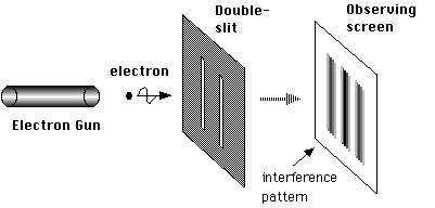
The setup of the electron diffraction double slit experiment.
Image credit NekoJaNekoJa on wikimedia commons released under GNU license.
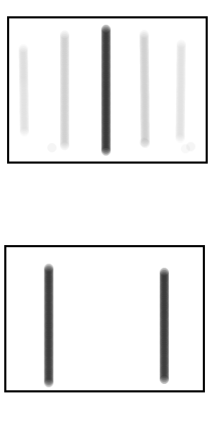
Top: The darker colours show areas more likely for the electron to hit the screen.
Bottom: For comparison, the areas where non-quantum physics predicts the electron would hit the screen. This is the case if we simply didn't know which slit the electron went through, but no diffraction occurs.
The reason an electron undergoes wavelike motion but a cricket ball (say) doesn’t is because the electron is small enough that it can go unobserved but with a cricket ball we will always be observing it either directly (we can see the cricket ball) or indirectly (we can feel the air it is pushing aside or feel the ever so faint tug of its gravitational attraction) and these observations continuously collapse the wave function into the solid object that we see.
If this description doesn’t raise a couple of questions for you then you’re not thinking hard enough! The two obvious questions with this interpretation are
Question 1) What counts as an observation?
Question 2) How does the electron decide where to appear when the wave function collapses?
The first question has been famously brought into focus by a thought experiment known as Shroedinger’s Cat, after Erwin Shroedinger who thought it up, and I’ll give a slightly modified version here. The experiment goes like this. A cat is sealed into a box. As the box lid is closed, an electron is released into the box and diffracted through two slits (this is the electron diffraction double slit experiment described above). If the electron lands on the left side of the screen then the cat is fine but if the electron lands on the right side of the screen then a vial of poison is broken which kills the cat.
The box is then reopened. The question is: Just before the box is opened, is the cat alive or dead?
According to the Bohr interpretation, since the lid is still on the box at this point, the electron is unobservable and therefore has not appeared on either the left or the right hand side of the screen but instead is still in the form of a wave function that is symmetrical across the screen. The cat is therefore also in the form of a wave function that is 50% dead and 50% alive. The cat remains in this wave like superposition and is neither dead or alive until the lid of the box is opened and the observation is made, at this point the wave function of the electron is collapsed and the electron is observed to have landed on either the left hand side of the screen (in which case the cat is alive) or on the right hand side of the screen (in which case the cat is dead).
Perhaps this is silly, you might think, and you’d be fairly reasonable for saying so. Why can’t the cat make the observation for instance? Does an observer have to be a human or will the cat do? Does the observer have to be conscious or could machine of some sort act as an observer? Perhaps a cat is simply too big and quantum mechanics applies only to microscopic objects like electrons.
The final objection there is easily dealt with. If we really want to say that quantum mechanics, fundamentally, only applies to the very small, then we have reverted back to the dualism that the Ancient Greeks had with one rule for the matter in the heavens and another rule for the matter on the Earth. It’s simply not a very good theory if you have to arbitrarily decide what kind of things (small things) are governed by it and which kind of things (large things) are not. Furthermore, where would this arbitrary cutoff occur and what would happen at the boundary- large objects are made up of smaller objects such as electrons after all? There are slightly more subtle versions of this answer, perhaps a certain amount of mass or a certain complexity of interaction causes the wave function to collapse spontaneously with no need to invoke the role of an observer, but it would still leave Question 2) from above, namely how does the collapsing object decide where on the wave function to appear.
What about the other objection- should cat count as an observer? Even if we had a really good reason to decide that only humans can count as observers we still run into problems.
Let's think about Shroedinger’s Cat experiment again [6], but this time when the scientist, let’s call her Alice, opens the box, she will make a note in her notebook of whether she observes the cat to be alive or dead. A short time later a second scientist, call him Bob, will enter the previously sealed lab and observe what Alice wrote in her notebook.
Since Bob knows that Alice will write “dead” in her notebook if she finds a dead cat and “alive” in her notebook if she finds a living cat, Bob can calculate the probability of what he will observe in the notebook before he looks, all he needs to do is calculate the probability that the cat is alive or dead when Alice opens the lid of the box. But, just as in the first experiment the cat was neither alive nor dead before the box was opened, now Alice can have written neither “alive” nor “dead” in her notebook until Bob opens the door to the lab. So now Alice, even though she is a human and therefore definitely a perfectly valid observer, manages to be in a superposition of states just as the cat must have been in a superposition of both alive and dead even if it was a valid observer.
You might at this point argue that whilst the cat was neither alive nor dead before the box was opened, once the box was opened then the notebook would contain either the word “alive” or “dead”, it’s just that Bob wouldn’t know which. But this misses the point that Shroedinger was making when he first made up the thought experiment and that is that the cat being neither alive nor dead is just a concrete, easy to visualise surrogate for the more abstract example of the electron being neither in one place or another on the screen. In the case of the electron (unlike the cat) simply not knowing at which point it is on the screen is different from it being a wave spread over the whole screen (as the Bohr interpretation understands it) since the probabilities of where the electron would be found would be different in each case, as we see in the Figure .If the electron went through one slit but you simply didn’t know which of the two slits then the most likely places to find the electron on the screen would be directly in front of one of the slits, you just wouldn’t know which. Whereas If the electron passes through both slits as a wave function then the most likely place to find the electron on the screen would be in the centre, which is actually the case. Therefore we know that an electron can exist in the form of a wave function. From our earlier reasoning, if an electron can exist in the form of a wave function then so can a cat and so can Alice; unless something causes the wave function to collapse.
An answer to this paradox is given in the PhD thesis of Hugh Everett, III entitled The Theory of the Universal Wave Function. The key thing that Everett noted was that the wave function collapse wasn’t strictly speaking necessary for the theory of quantum mechanics to work. Firstly, as we mentioned earlier, to avoid lapsing into dualism, the theory of quantum mechanics should be applicable to everything including observers. So an observer, such as a human, should be describable by a wave function. Therefore the act of observation should be viewed as a kind of interaction between two wave functions- the wave function of the observer and the wave function of the observed. Under the the Bohr interpretation, the definition of what is an observation and what isn’t an observation is crucial because it determines whether or not a wave function collapses. But Under Everett’s interpretation, the definition of an observation is not really important, it is just a particular kind of interaction between wave functions, one that provides the observer wave function with information on what state the observed wave function is in.
Likewise, what counts as an observer is now a fairly redundant question. An observer could be a conscious wave function such as a human or a cat or an unconscious wave function such as a machine.
So now let’s look again at the example of Shroedinger’s Cat with this new way of thinking. There is a wave function for the electron which is spread across the screen (as there is in the Bohr interpretation). The right hand part interacts with the wave function of the cat and causes that to split into a dead-part and an alive-part. When the box is opened these two parts interact with Alice’s wave function which splits and then in turn interacts with the notebook’s wave function etc. etc.
The lines between the different wave functions is blurred since the air between the cat and Alice would have a wave function and so would all of the photons that travel to Alice’s eyes and the interaction between these components would be constant. Therefore, instead of thinking of the wave functions as all being separate entities it might be more sensible to think of all of the wave functions as part of one Universal Wave Function. Part of this Universal Wave Function will represent the electron and part of it will represent Alice and so on. Rather than two wave functions interacting we now have one, self-interacting, Universal Wave Function.
It’s worth noting that in the Bohr interpretation, after the observation takes place, the cat is either alive or dead. But in the Everett interpretation, after the observation is made the Universal Wave Function contains both an alive cat and a dead cat as well as an Alice which has seen both.
I think that philosophically, this interpretation gives us a very different view of the world we live in. We look out and we see maybe a chair, a table, our hand and any number of other objects. From a very young age we learn to break down what we see into constituent objects. We say “there is the chair and there is the edge that it forms with the rest of the world” and so on. In particular we like to create a boundary between ourselves and the rest of the world. But these boundaries, even though useful to everyday life, can be seen to be entirely artificial. Even without appealing to the Universal Wave Function this is true to some extent. On a microscopic level you’d never be able to draw a sharp line between a chair and the rest of the world, for instance. Even if you defined what molecular structure of the wood composing the chair and defined the molecular structure of the air was you couldn’t draw a line between the two types of molecules and call one side “chair” and one side “the rest of the world& rdquo; because molecules just do not work that way. Under Bohr’s interpretation, a molecule only has a probability of being in a given place anyway. A given molecule of wood may be in the middle of a chair leg one moment but spontaneously several inches from the chair the next moment since it only ever appears at a given point on its wave function, at random, as it is observed. And under Everett’s interpretation the distinction is even more blurred since the chair is just a single part of the Universal Wave Function, as is the air around it.
This shows that it is very hard, and perhaps not worthwhile, to draw distinctions between different parts of the world at the deepest level. The chair is really just a part of the rest of the world and can’t be treated as something separate. And people are no different, still just parts of the Universal Wave Function that happen to be able to perceive other parts of the Universal Wave Function. To try and draw distinctions between yourself and the rest of the world, between yourself and other people, in the most absolute sense, is fairly futile.
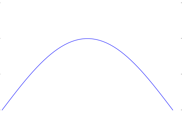
We saw that Everett defined an observation or measurement as any interaction between the two subsystems that reliably transferred information on the object being measured to the measuring apparatus. What we mean by information in this sense is predictability. If we are measuring the position of the particle, for instance, then information is the ability to precisely predict where it will be. Consider a wave function that is very spread out (Figure), we have very little information on this particle because it is hard to predict where the particle will be upon being measured. Conversely, if the wave function is very localised (Figure), then we have a lot of information because there is a high probability of the particle being found in a very small region.
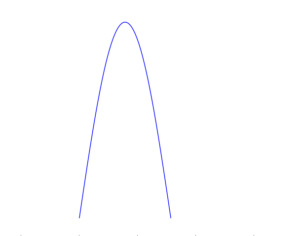
A very localised wave function. There is a high probability of finding the particle in the central region.
The sharp dichotomy of the Bohr interpretation, where making a measurement collapsed the wave function, has now been removed because it is possible to make a partial measurement which might increase the information we have on a system but only slightly. A very thorough measurement will give lots of information and therefore narrow down the location of the particle to a vanishingly small region of space. This is what was classically thought of as a measurement and conforms with the traditional point of view as a particle having a pointlike existence (rather than being wavelike and spread out over space) and in technical terms is called a “delta function”. This type of measurement is almost the only kind that can be performed in an everyday manner since large, everyday objects such as measuring devices with dials on and human beings are composed of so many millions of particles that even if each individual interaction was small the total would quickly add up. In fact, only very deliberate, laboratory experiments can perform partial measurements which barely disturb the wave function of an individual particle. This explains why everyday objects such as cricket balls and bullets, even specks of dirt, obey Newtonian physics and don’t display the quantum mechanical properties that individual particles can such as diffraction and interference.
As we just saw, when a strong enough interaction occurs, the wave functions of the interacting parts narrow down dramatically enough to be treated as point like particles. However, this cannot be the whole story, because as we saw in earlier chapters, waves have some very well defined properties that they must retain even if they are very sharply peaked.
The first property is called superposition or interference: we can add the values of two waves at each point together to get a combined wave. We mentioned this before in the chapter The Space and Time of Albert Einstein under The Nature of Light- Young’s Double Slit Experiment, but it is worth a very brief recap. Waves can be positive or negative at any point and two waves combined can end up adding together to make a point larger or subtracting from one another to make a point smaller. If two waves are completely opposite from one another then when one is subtracted from the other nothing is left; this is known as total destructive interference.
The second property to discuss is called phase. Look at a wave that repeats itself over and over again, see Figure. If we were to shift the whole wave along the horizontal axis this is known as changing its phase. If two identical waves are shifted relative to one another so that they can cancel out completely, the total destructive interference we just discussed, then we say that they are out of phase with one another.

It’s possible to stack waves together and add the results to obtain something that begins to resemble a particle. A demonstration of this summation can be seen below
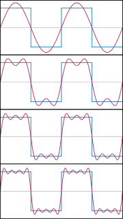
Waves being stacked together to form a rectangle. This process could be continued, to make a delta function, representing a particle at a definite position.
Image credit: Jim.belk, public domain.
As more and more waves are added to one another, the waves begin to cancel out in more and more places until the remaining wave becomes narrower and narrower and begins more and more to resemble a sharply defined delta function. This process can never be carried out perfectly, the waves you add always have some finite width so no matter how many you add together you’ll never quite end up with a delta function. Still we begin to see how something like a particle can emerge from summing together waves.
The physicist Richard Feynman looked for the reverse of this process. Can we take something like particles, existing in only one point in space, and add them together to get something that looks like a wave and explain the wavelike nature of particles this way? Let’s imagine we want to describe how a particle goes from a start point S to an end point F. We could describe the path taken by the particle using Newton’s Laws, we know how fast the particle would need to be travelling as it leaves S if it is to arrive at F, taking into account any forces such as gravity or an electric field.
What Feynman did was firstly to consider what would happen if the particle didn’t take the path prescribed by Newton’s Laws but took a different path instead. In fact, he considered every conceivable path between point S and point F, such as if the particle shot up into the air and then zig-zagged over to point F. Then he combined all of these paths together in much the same way that you can add together waves.
A way to imagine this process, not too far removed from the truth, is that when the particle leaves S it splits into an infinite number of particles. Each of these particles takes a different route, travelling through different points in space at different speeds, until eventually ending up at F. If this were the end of the story, these particles would recombine back into a single particle at F and would again look like a delta function on our diagram. But Feynman added one other ingredient which was that each path would acquire a phase based on the path taken. The path defined by Newton’s Laws is special because it conserves energy and momentum, so any increase in the particle’s speed is drawn out of the gravitational or electrical potentials around it. Any path that deviates from this will break these conservation laws, to a lesser or greater extent depending on the specifics of the path taken. The more a particle deviates from the conservation of energy the more rapidly its phase will change.
So our particle leaves S and splits into an infinite number of different particles each taking a unique path to F. The paths that come close to obeying the conservation laws only change phase very slowly, so these paths by and large reinforce each other. The paths that deviate greatly from the conservation laws change phase very rapidly and so by and large they cancel each other out and don’t contribute much. The amount of cancellation defines how probable it is to find the particle at F. If there is no cancellation we definitely find the particle there but as the paths cancel more and more the chance gets smaller and smaller.
We can repeat the calculation for other points in space other than F. We can examine the point just to the left or to the right of F. If we do so we find that each point in space will have a different value depending on how much the paths reaching it cancel with one another. The result is a probability at each point of finding the particle there. This is just the same as a wave function both in the general concept and in the precise mathematical result. We can see that the wavelike behaviour particles display arises when the particle explores the many different paths between S and F.
So far we have considered only a single particle but there’s no need to stop there and we can extend the approach to two, three or indeed any number of particles. With one particle we see the probability of going from a starting point S to a finishing point F by considering all possible paths for it. With many particles we see the probability of each particle going from its own particular starting point to its own particular finishing point along all possible paths. Another way of saying this is that we go from a particular starting configuration of particles to a particular finishing configuration of particles. Since each particle can take all possible paths, we must consider all possible configurations between the start and the finish (imagine all the particles were halfway between their start and finish along one of their many paths and you froze them in this state, that would also be a particular configuration of particles). In this way, what Feynman’s approach to quantum mechanics tells us is that we must consider how all possible configurations of a system can sum together given their different phases.
The two configurations at S and F as well as all of the intermediate configurations being considered can have different numbers and types of particles. This would occur when a particle emits one or more other particles, decays into two or more particles (which is radioactive decay) or when several particles combine to form a different particle (the reverse of radioactive decay).
Let’s consider a small number of particles, maybe a few dozen, going from a starting configuration S to a final configuration F. Imagine that all of the particles are electrons except for one which is a positron (don’t worry about the exact particles I’ve chosen, their properties are not important for this example it just helps the explanation to distinguish one of them from the others). If the positron is at quite some distance from all of the electrons in both configurations S and F we might expect the effect of the electrons on the positron’s path to be negligible- the path the positron takes is as though the electrons weren’t there.
But this is not the case. To find the probability of going from S to F we have to sum all the configurations of the system so we must consider configurations whereby some or all of the electrons appear very close to the positron for some or all of the journey between S and F and thereby affect the positron’s path. Such configurations are very unlikely, they require the electrons to shoot off towards the positron very rapidly and then return very rapidly before the positron reaches F. As we just discussed, we also need to consider configurations where the electrons emit particles or decay into other particles. Therefore we must also take into account configurations where these new daughter particles approach the positron and alter its path. Because we’re requiring all of our original electrons to still be present when we reach the final configuration F, these daughter particles must all eventually recombine with one another back into electrons. Therefore, although the daughter particles make their mark on the real world (by altering the positron’s path) we’ve required that they must disappear again in short order. These daughter particles are called virtual particles because they will never be measured like a “real” particle, despite affecting the motions of real particles.
There are many, many of these configurations with the electrons or their daughters near the positron but, because they deviate so much from the principle of conservation of energy and momentum, they largely cancel one another out when they sum together. However, there is not complete cancellation and residual effects are left over. These effects are sometimes called vacuum effects, because the space surrounding the positron’s path is empty (a vacuum) but still affects the particle. Vacuum effects, although small, are real and have been verified by experiment.
(A quick note for those who already know a little about this subject. It is often said that vacuum effects are caused by particle-antiparticle pairs “popping” into and out of existence in a very short time: being created and then annihilating. I don’t think this is a correct way to view the situation, since firstly the effects don’t rely on a particle-antiparticle pair and secondly this view implies that for a short duration the particle-antiparticle pair are real before annihilating which is not required under Path Integral or Canonical treatments of the situation see [5] Chapter 3, S 4.3. As far as I can this phrase was introduced into the lexicon by John Wheeler in 1957.)
If particles obey the laws of quantum mechanics and have a chance of appearing pretty much anywhere when you go looking for them, how come we don’t ever notice this in our everyday lives? We would never expect a cricket ball to diffract around a corner in the way we might expect an electron to.
The objects we encounter in our everyday lives our made up of a huge number of atoms. Nevermind cricket balls, there are hundreds of billions of atoms in a speck of household dust. The particles within this object are all bound together: they each interact by exchanging other particles and this means exchanging energy and momentum. This in turn means that for a particle within the object to deviate noticeably from Newton’s Laws it would have to stop conserving energy and momentum by a fairly considerable amount. A small number of particles might do this, but on average each particle deviates from Newton’s Laws very little and so the object as a whole, which in this case is the sum of its parts, obeys Newton’s Laws near perfectly.
(In the Bohr interpretation we would say that the interaction between particles counts as an observation and so the particle wave functions frequently collapse. Given the short time between ‘observations’ the wave functions never spread out much and so quantum mechanical behaviour is suppressed. For more in the universal wave function interpretation see [6] Chapter V S.1.)
As a brief recap, the sum over paths approach starts with an initial configuration of particles at a starting time and considers the possibility of a final configuration of particles being measured at a final time. As defined by Everett, this measurement is just an interaction between the particles which bestows information upon one subsystem which we define as the measuring apparatus (which could also be a conscious observer). In between these measurements, the particles are in a superposition of states as they take all possible paths between the two configurations. As mentioned, for large, everyday objects measurements occur almost constantly due to the huge numbers of particles involved and therefore the huge number of interactions. This means that these everyday objects have only a vanishingly small opportunity to exist in a superposition of states, but of course this behaviour manifests itself at the level of particle physics.
It might be tempting to ask what the position is of a particle (or all the particles) at some intermediate time between the initial and final states. Of course, the only way to find this out would be to actually perform a measurement, which would just make the intermediate time the new final time. Still, we might want to ask what the possibility is of a particle going from its initial position to its final position via some intermediate position as opposed to via any other route. If you calculate this, it turns out to be exactly the same probability as you calculate before, the intermediate position is accounted for since you already considered every possible configuration [7]. The only way that the result could be altered by the particle going via a specific intermediate position is if an interaction occurs there that somehow alters the configuration of the particles. A measurement will necessarily do this (altering the position of the dial on the measuring device and the brain of an observer watching it etc.), or something more destructive could be envisioned, such as the particle annihilating with another particle at that point. Any interaction that does occur there could be undone though: through random chance the dial on the measuring device could revert back to its previous position (along with the particles in the brain of the observer watching it) or a new particle could be created in the spot where the old one was annihilated. All these possibilities can be taken into account in the calculation, if a complete enough system is considered: a system with a measuring device and an observer and in which particles can be annihilated and created.
We have seen that the probability of going from our initial configuration to our final configuration is not altered by the inclusion of another configuration at an intermediate time. In fact, the other configuration does not need to be at an intermediate time, it could also be to the future of the final state: we can look at the possibility of going from our initial state way into the future and then back in time to our final state where the measurement is made [7]. How can this be? It sounds nonsensical and furthermore that it should violate causality. The fact is, the only thing that matters is the duration of time between the initial time and the final time when the measurement is performed. The numerical value we assign to the time coordinates of each configuration (e.g. 13:00 on 27th of April 2013 or 13:05 on 27th of April 2013) are fairly arbitrary. What is important from the point of view of causality is that the measurement at the initial configuration is performed before the measurement at the final configuration. From our previous discussion, we know that any measurement will alter the configuration, and that this alteration will be reflected in the measurement itself, in the position of the dial on the measuring device and in the particles in the observer’s brain etc. A record of the measurement is imprinted in the configuration of the particles itself.
When we say we are going from an initial configuration at a certain time to a final configuration at a certain time what we are saying is that we are going from an initial configuration which contains certain records to a final configuration that contains certain other records. The records at the final configuration will almost certainly include records from the initial configuration to some degree of fidelity. It’s conceivable that the total movement of particles between configurations would erase some records that were present in the initial configuration, but the probability of this happening to all the records is tremendously small unless a very large time was allowed between the initial and final configuration.
Basically, if the initial system has a large set of self-consistent records, the bulk of these are going to be carried over to later systems, simply adding to the store of records and memories. Of course, even if all the records were erased somehow, any observers in the system would be unaware that this had happened since they would have no record of the initial system. What we define as being “the past” is just a set of conceivable configurations that we have records for in our present configuration, just as fuzzy and indeterminate as the future.
In classical mechanics (i.e. non-quantum mechanics) every individual particle has a definite position at each instant in time and followed a set course completely determined by its momentum (and of course any collisions with other particles). This also meant that every particle was unique and distinguishable, in that it if you measured its position and momentum accurately you could trace its course back into the past and identify where it was.
All of this changes in quantum mechanics. Two particles of the same type (e.g. two electrons or two photons) can no longer be assigned definite trajectories [8]. Say that you have two electrons at points A1 and B1, and want to find the probability that some time later they will be at A2 and B2. Not only do you need to take into account that the electron at A1 goes to A2 while the electron and B1 goes to B2, but you also need to take into account that the two particles could swap over and the electron at A1 goes to B2 and the electron at B1 goes to A2.
This was is not the case in classical mechanics. At least in principle, when the particles are measured at A2 and B2, you could trace back the paths each particle had taken and declare at which point each particle started (i.e. which came from A1 and which came from B1). This also meant that at any intermediate time between measurements you could assign a position to them both.
But, in agreement to what we reasoned earlier, in quantum mechanics no intermediate positions can be assigned and only the instants of measurements have any real meaning. The fact you have to account for these extra paths where particles switchover means that the type of statistics used in quantum mechanics are quite different from those used in classical mechanics and lead to very different outcomes to experiments [C].
Key Points
Events that were impossible under Newtonian mechanics can have a small but non-zero chance of occurring in quantum mechanics.
This means that we no longer have a fully deterministic future. Even if we knew exactly what condition the universe was in at present, we could not perfectly predict the future.
Likewise, we do not have a fully deterministic past. Two different past states could have lead to the present state. In fact, all conceivable past states could have lead to the present state, although with varying probabilities.
Therefore, all we can say is how consistent different states of the universe are with being in our past, we do not have one definite history.
Footnotes
[A] Incidentally, Hertz’s experiments were among the first to demonstrate electromagnetic waves could be produced in air and were a strong validation for Maxwell’s electromagnetic theory .
[B] Einstein compared the entropy of radiation, as shown by Wien to the entropy of a gas and showed that the radiation could be thought of as discrete particles, using Planck’s formula with the discretisation of Planck’s constant. Crucially, Planck’s black body work gave a physical mechanism for how radiation is absorbed and emitted within a body, even if he was vague about it.
[C] A similar issue is one called gauge fixing. When calculating the probability to go from an initial configuration to a final configuration you take into account all the possible intermediate configurations. But just like switching two identical particles gives you the same results, so too does rotating your whole system. The final configuration where all particles are swung around by 45 degrees is just the same: all particles have the same distances and angles to one another.
This is evidence that quantum field theory is Machian, that it doesn’t seem to be nested in absolute space. But all the particles' movements between configurations takes place embedded in spacetime. What would happen if spacetime rotated? Would that need to be accounted for? What would it even rotate in?
This question was raised between Einstein and De Sitter in 1917. De Sitter showed that any movement of empty spacetime would not have an effect on observations, only movements of particles relative to the rest of the matter in the universe would have an effect.
References
[1] The Bumpy Road: Max Planck From radtion Theory to the quantum (1896 - 1906) / Massimiliano Badino
[2] Nobel Lecture / Max Planck available here.
[3] Nobel Lecture / Louis De Broglie available here.
[4] Address at the joint meeting of Section B of the American Association for the Advancement of Science and the American Physical Society on December 28, 1927 / Clinton Davisson.
[5] Student Friendly Quantum Field Theory / Robert D. Klauber
[6] The Theory of the Universal Wave Function / Hugh Everett, III
[7] See appendix.
[8] Studies in the History and Philosophy of Modern Physics / Simon Saunders